Repository navigation
L8 Kernel Spatial Convolution
This application is meant to demonstrate how spatial convolution works, giving you the chance to test with several kernels.
This application with generate a random image of 5x5 pixels. The values of each pixel are displayed on the left matrix, while a preview of the image is displayed at the bottom left, on the left side. In order to simplify the explanation of how a spatial convolution, we work only with monochromatic images.
The demonstration has two modes:
- Manual: You have to click the "Manual" button on the bottom right to move on to the next step of the demonstration.
- Automatic: By checking the "Auto" box on the bottom right, the steps will be done automatically. It takes a few seconds to start. You can control the speed at which the next step happens with the slide bar on the left.
With the "reset" button a new picture will be randomly generated and everything will go back to how it was.
To do a spatial convolution we need a kernel, with which we will be convoluting our image. That's what the 3x3 matrix on the bottom left is. You can change this kernel with the dropdown menu on the right. There are a few options to choose from. You can also make your own kernel.
We will be moving this kernel along the picture. This will be represented thanks to the colours green, blue and yellow of the kernel, which the cells of the image will light up as we apply the kernel to it.
A spatial convolution is done by placing the kernel on top of the picture, and then substituting the value of the pixel in the center by the sum of the results of multiplying the kernel with the pixels they overlap. Confusing, no? Well, that's what this application is for. Let's demonstrate.
First of all, we choose a kernel:
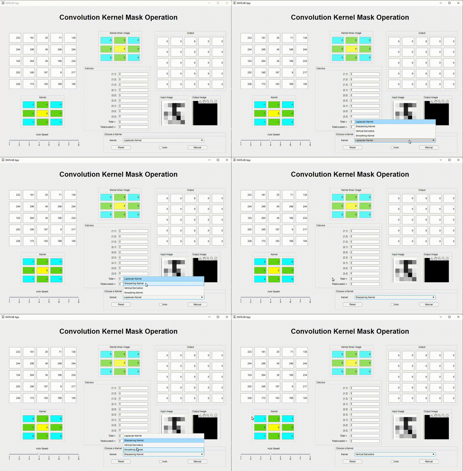
Then we click on Manual. As we can see several things light up and change:
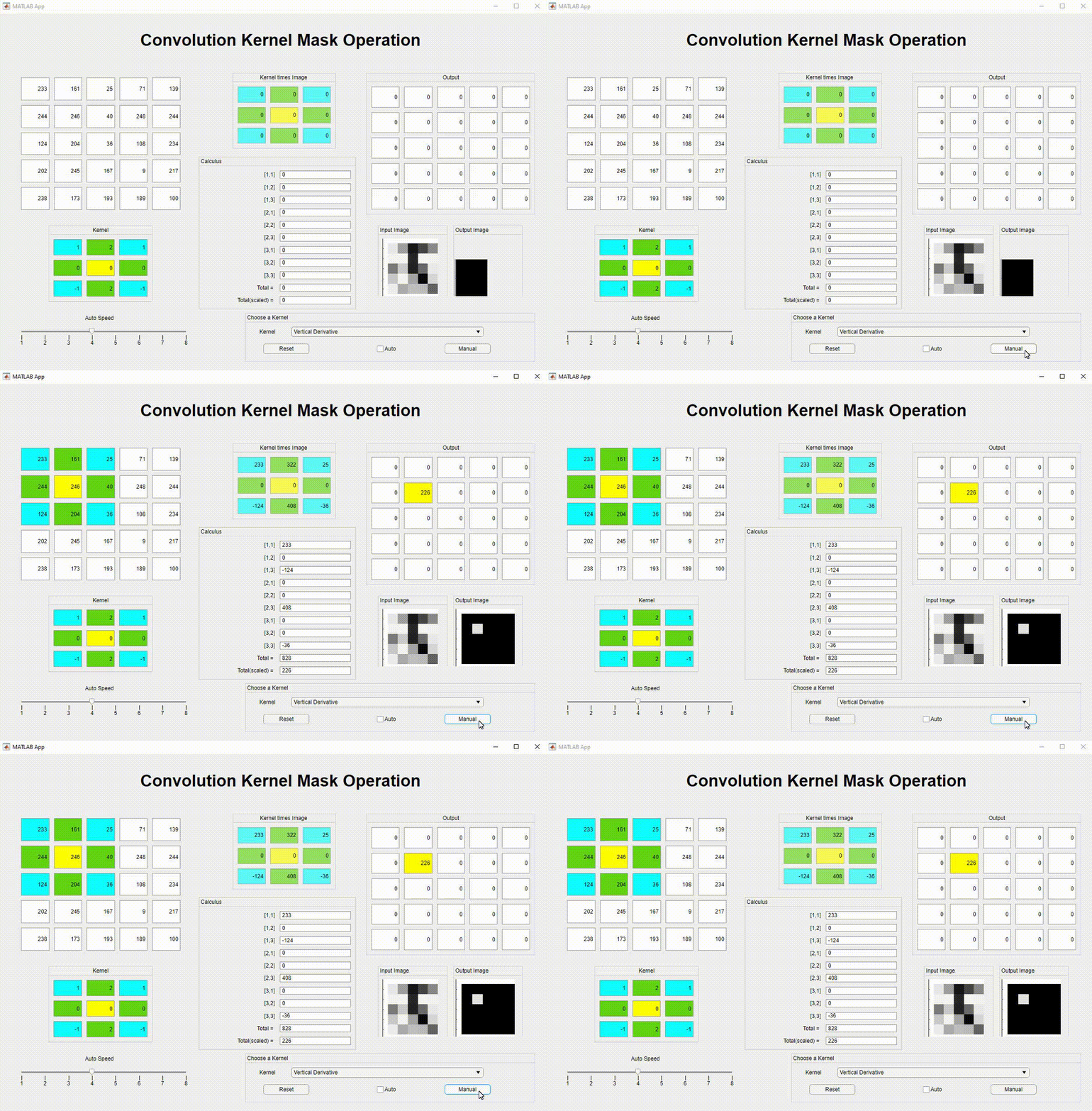
On the Image Matrix, the one on the left, we see the first 3x3 light up with the same colours of the kernel ( below it ). On it's right, we see the "Kernel times Image" matrix, which gives us the result of multiplying the position of the kernel by the pixel of the image it is over it. Another representation is underneath it in the calculus area. At the bottom of this area is the sum of all these results, which, once scaled (so that we get a value between 0 and 255), is then introduced in the position of the output image where the center of the kernel is. This is what we see in yellow on the output matrix, seen on the right. Below it, we can see that the output preview image now has a new pixel, the one we just created.
Once we click again on "Manual", the next step carries on, moving the kernel to the right. Once the kernel can be moved more to the right, it will move once down, and go back to the left. Repeating this until it has gone through all possible pixels. As it does so, the new image will be created.
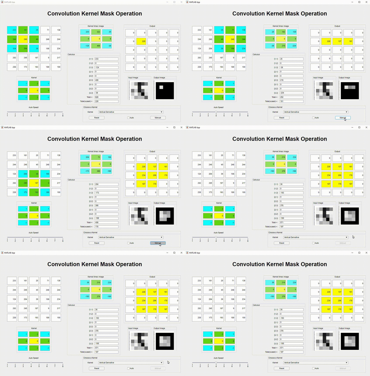
Spatial Convolution Effects vary greatly depending on the kernel used. But overall their effect is to smooth out images. This is turn can produce a loss of details.
I consider it important to notice how the image resulting from the convolution has less pixels than the one we started with. 5x5 becomes 3x3 with a kernel of 3x3.