This article represents only my personal views and is not related to the institution I work for.
TL;DR
Yesterday, NVIDIA announced the Groq 3 LPU and the corresponding LPX ComputeTray. However, we also noticed a complete absence of any mention of the Rubin CPX during this GTC. What is the logic behind this? How should we view this issue from the perspective of balancing various materials during a supply chain crunch? How is heterogeneous AFD (Attention FFN Disaggregation) implemented? How can the on-chip SRAM accommodate massive MoE models with over 1T parameters? What are the overall performance gains? What is the interconnect structure like?
By the way, the interconnect FPGA used in the system leverages some technologies from NetDAM, a project I worked on many years ago, which I also mentioned in my article #4 . I will elaborate on this later. Speaking of which, shouldn't Jensen pay up for that?

The table of contents for this article is as follows:
1. Groq 3 LPU Chip Architecture
1.1 Why Groq Needs Deterministic Execution
1.2 Groq 3 LPU Microarchitecture
1.3 Groq 3 ComputeTray Architecture
1.4 LPX Rack Structure
1.5 Fabric Expansion Logic
2. Vera Rubin + LPX
2.1 Why Inference Needs the Groq LPU
2.2 Detailed AFD Workflow
2.3 Speculative Decoding
3. Supply Chain Analysis of CPX and LPX
4. Future Outlook for the LPX System
1. Groq 3 LPU Chip Architecture
We have previously discussed Groq's microarchitecture in detail in the article #4 . Here, we will expand a bit on the topic of deterministic execution, which Groq has always emphasized.
1.1 Why Groq Needs Deterministic Execution
Traditional HPC systems and multi-core CPU/GPU architectures suffer from non-determinism due to dynamic sharing and contention for memory and network resources. The memory hierarchy of a GPGPU seems overly complex; while it simplifies programming to some extent, it often introduces uncontrollable factors. The sources of non-determinism mainly include several aspects:
- Dynamic instruction scheduling: Out-of-order execution cores change the completion order of instructions.
- Cache hierarchy: Cache hits/misses lead to uncertain memory access latencies.
- Dynamic network routing: Network congestion causes variations in packet delay and out-of-order arrivals.
- Shared memory arbitration: Multiple cores contend for the memory controller.
This poses a huge challenge for a very large-scale machine learning system. This non-determinism makes precise parallel coordination extremely difficult. In tightly-coupled parallel tasks, processor A does not know when processor B's data will arrive and can only wait through expensive synchronization mechanisms (like barriers and locks), leading to significant time wastage. Groq's philosophy is that instead of "managing" uncertainty with complex software in a non-deterministic system, it is better to build a deterministic system from the hardware level up.
Groq's solution: The core idea is to extend the determinism from within a single TSP (Tensor Streaming Processor) chip to the entire system composed of thousands of TSPs, through a meticulously designed set of hardware and software mechanisms. Deterministic execution includes the following two aspects:
- The network is no longer a "best-effort" dynamic system. Instead, the compiler plans all communication paths and timings at compile time, eliminating runtime network contention and congestion from the source.
- Runtime deskew instructions: The hardware provides special ISA instructions that allow software to periodically correct the minor time deviations caused by clock frequency drift in individual chips, thereby maintaining a macroscopic "lock-step" synchronization across the entire system.
Author note
This is why I have consistently emphasized the importance of Little's Law and Kingman's formula when modeling the entire system. Kingman's formula is an approximation for the mean waiting time in a general single-server queue model (G/G/1):
$$\mathbb E(W_q)=(\frac{\rho}{1-\rho})(\frac{c_a^2 +c_s^2}{2})\frac{1}{\mu}$$
where $\lambda$ is the arrival rate, $\mu$ is the service rate (the reciprocal of the average service time), and $\rho = \lambda / \mu$ is the system utilization. $c_a$ is the coefficient of variation (CV) of the arrival times, and $c_s$ is the CV of the service times. The CV is the standard deviation divided by the mean. We can then plot a graph based on $\rho / (1-\rho)$ for different coefficients of variation.

We notice that to shorten the average service waiting time of the entire system, it is necessary to further reduce the coefficients of variation for the network and computation ($c_a$, $c_s$). This is essential for the Expert Parallelism (EP) of the model. We will analyze this in detail later.
1.2 Groq 3 LPU Microarchitecture
The chip architecture of Groq 3 is shown in the figure below:

You might be wondering why it suddenly jumped to the third generation and what distinguishes its architecture from the first two.
The entire chip continues Groq's deterministic execution microarchitecture, including MXM (Matrix Multiplication Unit), VXM (Vector Computation Unit), MEM (Memory Function Unit), and SXM (Data Exchange Unit).

The MXM-SXM-MEM-VXM units form a pipeline, which is often referred to as a "SuperLane." Data flow is executed in parallel only in the east-west direction. In the north-south direction, it forms a parallel SIMD vector execution.

In the first-generation Groq architecture, each chip had 220MB of SRAM, forming a Scratchpad Memory with 80TB/s of bandwidth. There is no specific data for the second-generation chip, but we have seen Groq disclose that the main focus was on increasing the number of Serdes for chip interconnect and experimenting with building Scale-UP racks.

In the third generation, compared to the first, both the SRAM capacity and bandwidth have increased, supporting 500MB of SRAM capacity and 150TB/s of bandwidth. A rough estimate suggests that the VectorSize has been increased from 320B in the first generation to 768B, and the frequency has likely also improved as NVIDIA gains access to more advanced silicon technologies.
1.3 Groq 3 ComputeTray Architecture
From an interconnect perspective, Groq 3 supports 96 Chip-to-Chip (C2C) interconnect interfaces using 112G Serdes. This means a single chip supports 10Tbps of unidirectional bandwidth. An 8-chip ComputeTray, calculating with bidirectional memory bandwidth, achieves the 20TB/s ScaleUP bandwidth stated in the datasheet. The architecture of the entire ComputeTray is as follows:

The annotation for the physical photo is as follows:

The suspected internal interconnect structure of the ComputeTray is as follows:

The entire LPX rack supports 32 ComputeTrays. Therefore, each Groq 3 LPU needs to provide 31 C2C links to connect to other trays. Within the ComputeTray, an 800Gbps full-mesh connection is required, which would use 56 C2C links. 32 LPU C2C links are reserved on the front panel for interconnecting multiple LPX racks, with each LPU providing an average of 4 C2C links (400Gbps). The remaining 4 C2C links (400Gbps) are used to connect to the Fabric Expansion Logic FPGA. Additionally, the LPU and Fabric Expansion Logic require a PCIe connection to the Host CPU for control. Another BlueField-4 DPU or ConnectX-9 is used to connect to other front-end networks.
This interconnect method is also consistent with Groq's use of a Dragonfly topology. For a single Groq 3 LPU, 5.6Tbps of bandwidth is used for the full-mesh connection within the ComputeTray, 3.1Tbps is for the rack-level interconnect, 400Gbps is for cross-rack interconnect, and the remaining 400Gbps is for connecting to the Fabric Expansion Logic.
Below is the detailed datasheet for the ComputeTray:

Since each chip provides 1.2 PFLOPS of FP8 compute engine, a single ComputeTray has a total of 9.6 PFLOPS. A single Groq 3 LPU has 500MB of SRAM (with 150 TB/s of bandwidth), so an 8-chip configuration provides a total of 4GB of SRAM (with 1.2 PB/s of aggregate bandwidth). It is important to note that the Fabric Expansion Logic supports 256GB of DRAM, which is essential for supporting AFD on models with over 1T parameters. We will detail the specific function of this chip in a later section.
The Scale-UP bandwidth is 20 TB/s, which is calculated based on a single chip's 96 C2C (Chip-to-Chip) links running at 112 Gbps each. This equates to 10 Tbps unidirectional and 20 Tbps bidirectional per chip. The cumulative Scale-UP bandwidth for the 8-chip tray is 20 TB/s.
1.4 LPX Rack Structure
The entire rack contains 32 ComputeTrays. It is suspected that a CableTray is used for the backplane to connect the multiple ComputeTrays, and using only 112G Serdes should be less challenging than the CableTray in the Oberon-based cabinets.

Let's carefully examine these datasheet figures again. A single ComputeTray has 9.6 PFLOPS of FP8 compute, so 32 trays in a rack should total 307 PFLOPS. But the official promotion states 315 PFLOPS. So where do the extra 8 PFLOPS originate?
A single ComputeTray has 4GB of SRAM with 1.2 PB/s bandwidth. The entire rack would have 128GB of SRAM and an aggregate bandwidth of 38.4 PB/s. If we back-calculate from the stated 40 PB/s, each ComputeTray should have 1.25 PB/s. These data points have some inconsistencies, and we hope NVIDIA will clarify them.
The total of 256 LPUs in a rack amounts to 128GB of SRAM, but the aggregate bandwidth should be 38.4 PB/s. The Scale-UP Bandwidth is calculated simply by taking a single ComputeTray's 20TB/s and multiplying it by 32.
1.5 Fabric Expansion Logic
In late December 2025 I analyzed in detail how NVIDIA might integrate Groq's technology after the acquisition. During that time, I also mentioned a project of mine from 5 years ago, NetDAM. The narrow definition of NetDAM is Network Direct Attached Memory, meaning that attaching memory directly to an Ethernet controller via an ASIC falls into this category. And NVIDIA's Fabric Expansion Logic chip does exactly that. A comparison of the two chips is as follows:

In essence, this NVIDIA chip fully utilizes the technology from NetDAM developed years ago. If one were to argue that connecting to other processors instead of standard PCIe/CXL is a difference, NetDAM had already claimed direct connection to various chips.

Shouldn't Jensen send some money my way?
Returning to the topic, why does NVIDIA need to place this chip on the LPX ComputeTray for fabric expansion? First, the entire Groq processing domain is deterministic, whereas networks are typically affected by congestion and latency/jitter. As the NetDAM paper states, a "dam" is needed at the host boundary to absorb inter-host bursts and jitter and provide deterministic memory access to the internal system.
We will expand on how this chip is used in detail when we discuss AFD in a later section.
2. Vera Rubin + LPX
First, you must be wondering: since the GPU is already a heterogeneous accelerator, why add another heterogeneous chip, the Groq LPU?
2.1 Why Inference Needs the Groq LPU?
First, we need to analyze the entire workload in detail, especially the workload of Agentic LLM inference.
Agentic LLM Workload Characteristics
Modern Agentic LLMs are often given a complex task, like "write a web scraper to fetch weather data." The agent will independently search for information online, write code, run the code, and debug errors. This process can involve dozens or even hundreds of steps. Although each individual tool call or feedback is short (usually a few hundred tokens), the context accumulates with each turn, growing to extremely long lengths. This means the workload characteristics of an agentic LLM are a very long context length (>100K) and multi-turn interactions. Each interaction proceeds as follows:
- The model generates 1000-2000 tokens in the Decoding phase, which may include tool calls.
- The Agent executes the tool calls returned by the model and returns the results, typically a few hundred tokens.
- The inference engine appends the Agent's results to the context and performs a Prefill operation.
- After the Prefill is complete, the model enters the Decoding phase again to generate new tool calls.
Prefill Workload
As the context grows longer over multiple turns, it actually places a higher demand on memory capacity. Therefore, we can consider this phase to be constrained by Memory Capacity Bound. Of course, the prefill phase itself is also a Compute Bound process.
Decode Workload
In the Decoding phase, Attention-related computations still need to maintain the entire context, so there is also a Memory Capacity Bound constraint. Due to memory capacity limitations, many operations run at very small batch sizes. Furthermore, in the MoE phase, a single token typically requires 8 experts to participate in the computation, and loading these expert parameters also causes significant memory access. Therefore, this phase is also a Memory Bandwidth Bound process.
In summary:
- Prefill phase: Compute Bound + Memory Capacity Bound
- Decode phase: Memory Capacity Bound (Attention Block Only) + Memory Bandwidth Bound
On the other hand, the traditional Tokens Per Second (TPS) SLO is designed for chat scenarios, tailored to human reading speed. For an agent, it takes only a very short time to read the tool calls returned by the model. Therefore, in multi-turn scenarios, we need to significantly increase the TPS of the Decode phase to accelerate the overall execution time of the agent. This means the SLO for an "AI Factory" requires both high overall throughput (TPS per MW) and higher per-user TPS (TPS per User).

Let's elaborate a bit on why agents need high per-user TPS. Assume a Time To First Token (TTFT) of 3s, and an agent's execution time per turn is 100ms. If TPS = 20, and we assume the Decode phase requires 500 tokens, the Decode time would be 25s. If an agent task needs 10 turns, the total execution time would be (3 + 25 + 0.1) * 10 = 281s. If TPS = 100, the Decode time becomes 5s, and the total execution time is 81s. Therefore, 100 TPS or 150 TPS will become the minimum SLO requirement for Agentic LLMs. NVIDIA's blog also touched upon this issue:

If we were to use only HBM-based Rubin GPUs, we would have to consider GPU efficiency, especially in the Decoding phase where small batch sizes lead to low GEMM efficiency. This often means sacrificing some per-user latency to achieve higher throughput with a relatively larger batch size. Such a trade-off is unacceptable for Agentic LLMs. Of course, we could use a very low batch size to serve users who need extreme high TPS, but the resulting low overall throughput would lead to extremely high costs for the AI Factory, which would then be passed on to the users.

If we were to use only SRAM-based Groq LPUs, although such processors can achieve extremely low per-session inference latency (outputting over 1000 TPS), the limited SRAM capacity of the entire system results in poor concurrency, meaning the overall throughput still does not meet the needs of an AI Factory.

Let's fully compare the characteristics of the two types of chips: Rubin has higher compute power and larger memory capacity, while Groq has much higher memory bandwidth.

A very natural idea emerges: how to combine the two chips. Rubin's massive compute and large HBM capacity can address the constraints of Prefill. At the same time, its HBM capacity and compute power are also fine for handling the Attention calculations in the Decoding phase. The FFN part of the Decoding phase can then be offloaded to the Groq 3 LPU, which has much higher bandwidth. As shown in the figure:

This collaborative approach should theoretically lead to significant performance improvements, as shown below:
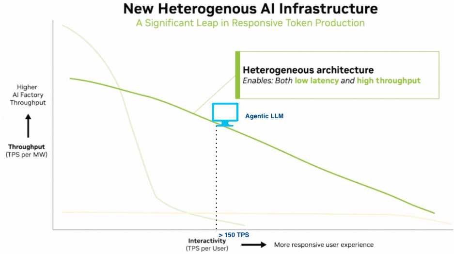
However, we should note that this is a theoretical trade-off. What are the actual performance gains?
2.2 Detailed AFD Workflow
NVIDIA's official blog only provides a simple diagram for AFD:

Let's take DeepSeek-V3's MoE as an example. A single expert has 44.05M parameters, which is 44.05MB using FP8. Each layer has 256 routed experts and 1 shared expert. Across 58 layers, the total parameters require 656.6GB. If we were to rely solely on the SRAM of the Groq 3 LPU, a single rack with 128GB would be unable to hold an MoE model with over 1T parameters. Therefore, a common view among networking professionals is that it would require 10 racks and 2560 cards to store so many expert parameters. However, the key to solving this problem lies in the 256 GB DRAM on the Fabric Expansion Logic.
Now let's estimate the computation time for a single expert. Constrained by the Groq 3's 1.2 PFLOPS compute and 150 TB/s SRAM bandwidth, this kernel is Memory Bandwidth Bound. The total data size is 264MB, and the memory access latency is 1.68 us. This means the entire operator computation time is about 2us.
The Groq 3 has a FIFO for caching tokens, as shown below:

The entire data interaction flow is as follows:

First, the Rubin GPU needs to dispatch tokens to the FIFO on the Groq 3 using IBGDA (InfiniBand GPUDirect Async). IBGDA must be used here because using IBRC (InfiniBand Reliable Connected) would result in higher latency. Let's assume an ideal scenario where the transfer takes only 3us, the Groq 3 LPU computation takes 2us, and the data return write to Rubin also takes 3us. The entire process takes about 10us.
Next, let's discuss the Expert Parallelism (EP) strategy. Since an LPX rack has 256 Groq 3 LPUs, it is possible to achieve EP-256. The shared expert can be computed on the Rubin GPU itself. There are also some considerations for expert load balancing; the computation time for certain experts might need to include the serving queue time on the Groq 3 LPU. For now, let's assume an optimal end-to-end time of 15us. And let's assume that within the Groq cluster, we can use a few LPUs to handle the ep-combine kernel. For simplicity, we'll assume the total EP communication and FFN computation time is 20us.
A particularly important issue to note is that with such a low computation and communication latency, potential network congestion (jitter caused by incast) and latency jitter from hash collisions need special handling. Otherwise, network jitter will further impact the completion time.
Now, let's use a tool I previously developed, ShallowSim, to simulate the MLA (Multi-head Latent Attention) computation time on Rubin. Since the expert parameters are stored on the Groq 3 LPUs, Rubin has enough memory to store a much longer KV Cache. However, to achieve lower latency, the batch size on Rubin needs to be smaller. Let's take Batch Size = 16 as an example for simulation. The table below shows the MLA operator time and the TPS calculated based on 61 layers plus the FFN time (20us):
| Context Length |
1K |
4K |
8K |
32K |
64K |
128K |
| MLA |
67us |
72us |
79us |
125us |
225us |
400us |
| TPS |
188 |
178 |
165 |
113 |
67 |
39 |
If we calculate with Batch Size = 4:
| Context Length |
1K |
4K |
8K |
32K |
64K |
128K |
| MLA |
66us |
67us |
69us |
80us |
94us |
124us |
| TPS |
190 |
188 |
184 |
163 |
143 |
113 |
This is the TPS without Speculative Decoding. If we enable it, we can assume a 2-3x increase in TPS in a small batch size scenario. This means that if we want to meet an end-to-end TPS > 100, the entire forward computation latency needs to be kept within 30ms (TPS = 33, at which point the time per layer is about 490us).
Compared to a pure Rubin solution, if we use traditional two-batch overlap, the TPS would be roughly halved, forcing the use of an even smaller batch size to meet the TPS SLO. This is why Jensen talks about a 2x throughput benefit.

However, there is another bottleneck we haven't considered. Due to the limited SRAM capacity of the Groq 3 LPU, we cannot place all experts for EP-256. Therefore, we need to load a subset of layers' experts into the Groq-3 LPU, compute one layer, and then prefetch the expert parameters for the next layer from the DDR on the Fabric Expansion Logic. Assuming DDR5-6400, the bandwidth of a single memory stick is 51.2GB/s. Four sticks provide a total of 204.8GB/s, which is 1.6Tbps of maximum bandwidth connecting to the Groq 3 LPUs. This averages out to only 200Gbps of bandwidth per Groq LPU. If we use MRDIMM 12800, the average bandwidth per Groq LPU becomes 400Gbps. Transferring one expert's 44MB of parameters at 400Gbps would take 800us. Therefore, this bottleneck still requires multiple LPX-Racks to alleviate.
On another note, since the acquisition of Groq is recent, designing a dedicated Fabric Expansion Logic ASIC would take a long time. Thus, the current time-to-market solution has to be an FPGA. A single FPGA is limited by the total number of Serdes and DDR controllers. I estimate that when NVIDIA delivers the LPX ComputeTray, it might require 2 FPGAs providing a total of 8 channels of DDR5 controllers to meet the latency requirements for asynchronously loading expert parameters.
2.3 Speculative Decoding
NVIDIA's official blog also describes another use case for the Groq LPU: speculative decoding.

Let's take the Eagle-3 algorithm as an example. The speculative decoding model is typically a very small-scale model. The algorithm is shown in the figure below:

Suppose the target model has already generated "How can I". When generating "I", we not only note down this word but also extract the early, middle, and late-stage thought processes (low, mid, and high-level features) related to "How" and "can" from the target model. Then, we merge these features from different stages to get more refined features, $g_{how}$ and $g_{can}$.
Next, we use a draft model. We feed it the refined features we just obtained, $g_{how}, g_{can}$, along with the information of the newly generated word "I" (its word embedding $e_I$). After some computation, it produces an intermediate result $a_I$. This result, when passed through the target model's "translator" (LM head), allows it to guess that the next word is "do".
Now we want to guess the word after "do". However, "do" is just our guess and hasn't been confirmed by the target large model, so we cannot get its corresponding "refined feature" $g_{do}$. What do we do? EAGLE-3 uses a clever alternative: it directly uses the intermediate result $a_I$ generated in the previous step to pretend it's the refined feature of "I", $g_I$. Then, it feeds this pretended $g_I$ (which is $a_I$) along with the information of the newly guessed word "do" ($e_{do}$) to the small assistant. After another round of computation, it gets $a_{do}$, and subsequently guesses the next word, "it".
The entire Eagle-3 draft model is very small, typically only 3-4GB, so it can be fully placed on the Groq 3 LPUs. Since the entire LPX rack has 256 cards, we can actually place multiple copies of the draft model to increase parallel processing.
3. Supply Chain Analysis of CPX and LPX
When both HBM and DDR supplies are extremely tight, and power and data center availability in North America are also constrained, how to generate more tokens under limited supply chain support becomes a critical problem for Jensen to solve. The rising price of DDR, combined with the significant memory demands of Agentic LLMs on CPU instances, means the cost difference between Rubin CPX and Rubin+HBM is rapidly shrinking. Furthermore, Rubin CPX lacks NVLink. From the perspectives of data center footprint, power consumption, and impact on the DDR supply chain, its existence is no longer justified.
Then, using Groq 3 LPUs for some decoding nodes can also reduce the dependency on HBM and lower power consumption.
We also note that the Vera CPU and the BF4 STS storage server are also built into rack-level high-density solutions. This can further reduce the data center footprint and share some liquid cooling/power supply chain components to further lower costs.
Under these overall supply chain constraints, although it seems like every product form is adopting a mainframe-like rack scale, we can understand that Jensen is striving to address supply shortages to cope with the explosive growth in token usage.
4. Future Outlook for the LPX System
As we saw in the second chapter, the Fabric Expansion Logic (FEL) is a temporary time-to-market solution. I personally estimate that significant benefits for models with >1T parameters will only become apparent with Groq 3.5 (L35) supporting nvfp4. Otherwise, loading parameters from the FEL's DDR into the Groq 3 LPU will still be constrained by bandwidth. Using nvfp4 can halve the bandwidth requirement.
Of course, the ultimate solution will have to wait for the Feynman generation, which will involve switching the Groq LPU's C2C bus to NVLink, and integrating FEL functionality into the CX10 switch while supporting DDR6 to meet the demand.

This article represents only my personal views and is not related to the institution I work for.
TL;DR
Yesterday, NVIDIA announced the Groq 3 LPU and the corresponding LPX ComputeTray. However, we also noticed a complete absence of any mention of the Rubin CPX during this GTC. What is the logic behind this? How should we view this issue from the perspective of balancing various materials during a supply chain crunch? How is heterogeneous AFD (Attention FFN Disaggregation) implemented? How can the on-chip SRAM accommodate massive MoE models with over 1T parameters? What are the overall performance gains? What is the interconnect structure like?
By the way, the interconnect FPGA used in the system leverages some technologies from NetDAM, a project I worked on many years ago, which I also mentioned in my article #4 . I will elaborate on this later. Speaking of which, shouldn't Jensen pay up for that?
The table of contents for this article is as follows:
1. Groq 3 LPU Chip Architecture
We have previously discussed Groq's microarchitecture in detail in the article #4 . Here, we will expand a bit on the topic of deterministic execution, which Groq has always emphasized.
1.1 Why Groq Needs Deterministic Execution
Traditional HPC systems and multi-core CPU/GPU architectures suffer from non-determinism due to dynamic sharing and contention for memory and network resources. The memory hierarchy of a GPGPU seems overly complex; while it simplifies programming to some extent, it often introduces uncontrollable factors. The sources of non-determinism mainly include several aspects:
This poses a huge challenge for a very large-scale machine learning system. This non-determinism makes precise parallel coordination extremely difficult. In tightly-coupled parallel tasks, processor A does not know when processor B's data will arrive and can only wait through expensive synchronization mechanisms (like barriers and locks), leading to significant time wastage. Groq's philosophy is that instead of "managing" uncertainty with complex software in a non-deterministic system, it is better to build a deterministic system from the hardware level up.
Groq's solution: The core idea is to extend the determinism from within a single TSP (Tensor Streaming Processor) chip to the entire system composed of thousands of TSPs, through a meticulously designed set of hardware and software mechanisms. Deterministic execution includes the following two aspects:
Author note
This is why I have consistently emphasized the importance of Little's Law and Kingman's formula when modeling the entire system. Kingman's formula is an approximation for the mean waiting time in a general single-server queue model (G/G/1):
where$\lambda$ is the arrival rate, $\mu$ is the service rate (the reciprocal of the average service time), and $\rho = \lambda / \mu$ is the system utilization. $c_a$ is the coefficient of variation (CV) of the arrival times, and $c_s$ is the CV of the service times. The CV is the standard deviation divided by the mean. We can then plot a graph based on $\rho / (1-\rho)$ for different coefficients of variation.
We notice that to shorten the average service waiting time of the entire system, it is necessary to further reduce the coefficients of variation for the network and computation ($c_a$ , $c_s$ ). This is essential for the Expert Parallelism (EP) of the model. We will analyze this in detail later.
1.2 Groq 3 LPU Microarchitecture
The chip architecture of Groq 3 is shown in the figure below:
You might be wondering why it suddenly jumped to the third generation and what distinguishes its architecture from the first two.
The entire chip continues Groq's deterministic execution microarchitecture, including MXM (Matrix Multiplication Unit), VXM (Vector Computation Unit), MEM (Memory Function Unit), and SXM (Data Exchange Unit).
The MXM-SXM-MEM-VXM units form a pipeline, which is often referred to as a "SuperLane." Data flow is executed in parallel only in the east-west direction. In the north-south direction, it forms a parallel SIMD vector execution.

In the first-generation Groq architecture, each chip had 220MB of SRAM, forming a Scratchpad Memory with 80TB/s of bandwidth. There is no specific data for the second-generation chip, but we have seen Groq disclose that the main focus was on increasing the number of Serdes for chip interconnect and experimenting with building Scale-UP racks.

In the third generation, compared to the first, both the SRAM capacity and bandwidth have increased, supporting 500MB of SRAM capacity and 150TB/s of bandwidth. A rough estimate suggests that the VectorSize has been increased from 320B in the first generation to 768B, and the frequency has likely also improved as NVIDIA gains access to more advanced silicon technologies.
1.3 Groq 3 ComputeTray Architecture
From an interconnect perspective, Groq 3 supports 96 Chip-to-Chip (C2C) interconnect interfaces using 112G Serdes. This means a single chip supports 10Tbps of unidirectional bandwidth. An 8-chip ComputeTray, calculating with bidirectional memory bandwidth, achieves the 20TB/s ScaleUP bandwidth stated in the datasheet. The architecture of the entire ComputeTray is as follows:
The annotation for the physical photo is as follows:
The suspected internal interconnect structure of the ComputeTray is as follows:
The entire LPX rack supports 32 ComputeTrays. Therefore, each Groq 3 LPU needs to provide 31 C2C links to connect to other trays. Within the ComputeTray, an 800Gbps full-mesh connection is required, which would use 56 C2C links. 32 LPU C2C links are reserved on the front panel for interconnecting multiple LPX racks, with each LPU providing an average of 4 C2C links (400Gbps). The remaining 4 C2C links (400Gbps) are used to connect to the Fabric Expansion Logic FPGA. Additionally, the LPU and Fabric Expansion Logic require a PCIe connection to the Host CPU for control. Another BlueField-4 DPU or ConnectX-9 is used to connect to other front-end networks.
This interconnect method is also consistent with Groq's use of a Dragonfly topology. For a single Groq 3 LPU, 5.6Tbps of bandwidth is used for the full-mesh connection within the ComputeTray, 3.1Tbps is for the rack-level interconnect, 400Gbps is for cross-rack interconnect, and the remaining 400Gbps is for connecting to the Fabric Expansion Logic.
Below is the detailed datasheet for the ComputeTray:

Since each chip provides 1.2 PFLOPS of FP8 compute engine, a single ComputeTray has a total of 9.6 PFLOPS. A single Groq 3 LPU has 500MB of SRAM (with 150 TB/s of bandwidth), so an 8-chip configuration provides a total of 4GB of SRAM (with 1.2 PB/s of aggregate bandwidth). It is important to note that the Fabric Expansion Logic supports 256GB of DRAM, which is essential for supporting AFD on models with over 1T parameters. We will detail the specific function of this chip in a later section.
The Scale-UP bandwidth is 20 TB/s, which is calculated based on a single chip's 96 C2C (Chip-to-Chip) links running at 112 Gbps each. This equates to 10 Tbps unidirectional and 20 Tbps bidirectional per chip. The cumulative Scale-UP bandwidth for the 8-chip tray is 20 TB/s.
1.4 LPX Rack Structure
The entire rack contains 32 ComputeTrays. It is suspected that a CableTray is used for the backplane to connect the multiple ComputeTrays, and using only 112G Serdes should be less challenging than the CableTray in the Oberon-based cabinets.
Let's carefully examine these datasheet figures again. A single ComputeTray has 9.6 PFLOPS of FP8 compute, so 32 trays in a rack should total 307 PFLOPS. But the official promotion states 315 PFLOPS. So where do the extra 8 PFLOPS originate?
A single ComputeTray has 4GB of SRAM with 1.2 PB/s bandwidth. The entire rack would have 128GB of SRAM and an aggregate bandwidth of 38.4 PB/s. If we back-calculate from the stated 40 PB/s, each ComputeTray should have 1.25 PB/s. These data points have some inconsistencies, and we hope NVIDIA will clarify them.
The total of 256 LPUs in a rack amounts to 128GB of SRAM, but the aggregate bandwidth should be 38.4 PB/s. The Scale-UP Bandwidth is calculated simply by taking a single ComputeTray's 20TB/s and multiplying it by 32.
1.5 Fabric Expansion Logic
In late December 2025 I analyzed in detail how NVIDIA might integrate Groq's technology after the acquisition. During that time, I also mentioned a project of mine from 5 years ago, NetDAM. The narrow definition of NetDAM is Network Direct Attached Memory, meaning that attaching memory directly to an Ethernet controller via an ASIC falls into this category. And NVIDIA's Fabric Expansion Logic chip does exactly that. A comparison of the two chips is as follows:
In essence, this NVIDIA chip fully utilizes the technology from NetDAM developed years ago. If one were to argue that connecting to other processors instead of standard PCIe/CXL is a difference, NetDAM had already claimed direct connection to various chips.
Shouldn't Jensen send some money my way?
Returning to the topic, why does NVIDIA need to place this chip on the LPX ComputeTray for fabric expansion? First, the entire Groq processing domain is deterministic, whereas networks are typically affected by congestion and latency/jitter. As the NetDAM paper states, a "dam" is needed at the host boundary to absorb inter-host bursts and jitter and provide deterministic memory access to the internal system.
We will expand on how this chip is used in detail when we discuss AFD in a later section.
2. Vera Rubin + LPX
First, you must be wondering: since the GPU is already a heterogeneous accelerator, why add another heterogeneous chip, the Groq LPU?
2.1 Why Inference Needs the Groq LPU?
First, we need to analyze the entire workload in detail, especially the workload of Agentic LLM inference.
Agentic LLM Workload Characteristics
Modern Agentic LLMs are often given a complex task, like "write a web scraper to fetch weather data." The agent will independently search for information online, write code, run the code, and debug errors. This process can involve dozens or even hundreds of steps. Although each individual tool call or feedback is short (usually a few hundred tokens), the context accumulates with each turn, growing to extremely long lengths. This means the workload characteristics of an agentic LLM are a very long context length (>100K) and multi-turn interactions. Each interaction proceeds as follows:
Prefill Workload
As the context grows longer over multiple turns, it actually places a higher demand on memory capacity. Therefore, we can consider this phase to be constrained by Memory Capacity Bound. Of course, the prefill phase itself is also a Compute Bound process.
Decode Workload
In the Decoding phase, Attention-related computations still need to maintain the entire context, so there is also a Memory Capacity Bound constraint. Due to memory capacity limitations, many operations run at very small batch sizes. Furthermore, in the MoE phase, a single token typically requires 8 experts to participate in the computation, and loading these expert parameters also causes significant memory access. Therefore, this phase is also a Memory Bandwidth Bound process.
In summary:
On the other hand, the traditional Tokens Per Second (TPS) SLO is designed for chat scenarios, tailored to human reading speed. For an agent, it takes only a very short time to read the tool calls returned by the model. Therefore, in multi-turn scenarios, we need to significantly increase the TPS of the Decode phase to accelerate the overall execution time of the agent. This means the SLO for an "AI Factory" requires both high overall throughput (TPS per MW) and higher per-user TPS (TPS per User).
Let's elaborate a bit on why agents need high per-user TPS. Assume a Time To First Token (TTFT) of 3s, and an agent's execution time per turn is 100ms. If TPS = 20, and we assume the Decode phase requires 500 tokens, the Decode time would be 25s. If an agent task needs 10 turns, the total execution time would be (3 + 25 + 0.1) * 10 = 281s. If TPS = 100, the Decode time becomes 5s, and the total execution time is 81s. Therefore, 100 TPS or 150 TPS will become the minimum SLO requirement for Agentic LLMs. NVIDIA's blog also touched upon this issue:
If we were to use only HBM-based Rubin GPUs, we would have to consider GPU efficiency, especially in the Decoding phase where small batch sizes lead to low GEMM efficiency. This often means sacrificing some per-user latency to achieve higher throughput with a relatively larger batch size. Such a trade-off is unacceptable for Agentic LLMs. Of course, we could use a very low batch size to serve users who need extreme high TPS, but the resulting low overall throughput would lead to extremely high costs for the AI Factory, which would then be passed on to the users.
If we were to use only SRAM-based Groq LPUs, although such processors can achieve extremely low per-session inference latency (outputting over 1000 TPS), the limited SRAM capacity of the entire system results in poor concurrency, meaning the overall throughput still does not meet the needs of an AI Factory.
Let's fully compare the characteristics of the two types of chips: Rubin has higher compute power and larger memory capacity, while Groq has much higher memory bandwidth.
A very natural idea emerges: how to combine the two chips. Rubin's massive compute and large HBM capacity can address the constraints of Prefill. At the same time, its HBM capacity and compute power are also fine for handling the Attention calculations in the Decoding phase. The FFN part of the Decoding phase can then be offloaded to the Groq 3 LPU, which has much higher bandwidth. As shown in the figure:
This collaborative approach should theoretically lead to significant performance improvements, as shown below:
However, we should note that this is a theoretical trade-off. What are the actual performance gains?
2.2 Detailed AFD Workflow
NVIDIA's official blog only provides a simple diagram for AFD:
Let's take DeepSeek-V3's MoE as an example. A single expert has 44.05M parameters, which is 44.05MB using FP8. Each layer has 256 routed experts and 1 shared expert. Across 58 layers, the total parameters require 656.6GB. If we were to rely solely on the SRAM of the Groq 3 LPU, a single rack with 128GB would be unable to hold an MoE model with over 1T parameters. Therefore, a common view among networking professionals is that it would require 10 racks and 2560 cards to store so many expert parameters. However, the key to solving this problem lies in the 256 GB DRAM on the Fabric Expansion Logic.
Now let's estimate the computation time for a single expert. Constrained by the Groq 3's 1.2 PFLOPS compute and 150 TB/s SRAM bandwidth, this kernel is Memory Bandwidth Bound. The total data size is 264MB, and the memory access latency is 1.68 us. This means the entire operator computation time is about 2us.
The Groq 3 has a FIFO for caching tokens, as shown below:

The entire data interaction flow is as follows:
First, the Rubin GPU needs to dispatch tokens to the FIFO on the Groq 3 using IBGDA (InfiniBand GPUDirect Async). IBGDA must be used here because using IBRC (InfiniBand Reliable Connected) would result in higher latency. Let's assume an ideal scenario where the transfer takes only 3us, the Groq 3 LPU computation takes 2us, and the data return write to Rubin also takes 3us. The entire process takes about 10us.
Next, let's discuss the Expert Parallelism (EP) strategy. Since an LPX rack has 256 Groq 3 LPUs, it is possible to achieve EP-256. The shared expert can be computed on the Rubin GPU itself. There are also some considerations for expert load balancing; the computation time for certain experts might need to include the serving queue time on the Groq 3 LPU. For now, let's assume an optimal end-to-end time of 15us. And let's assume that within the Groq cluster, we can use a few LPUs to handle the ep-combine kernel. For simplicity, we'll assume the total EP communication and FFN computation time is 20us.
A particularly important issue to note is that with such a low computation and communication latency, potential network congestion (jitter caused by incast) and latency jitter from hash collisions need special handling. Otherwise, network jitter will further impact the completion time.
Now, let's use a tool I previously developed, ShallowSim, to simulate the MLA (Multi-head Latent Attention) computation time on Rubin. Since the expert parameters are stored on the Groq 3 LPUs, Rubin has enough memory to store a much longer KV Cache. However, to achieve lower latency, the batch size on Rubin needs to be smaller. Let's take Batch Size = 16 as an example for simulation. The table below shows the MLA operator time and the TPS calculated based on 61 layers plus the FFN time (20us):
If we calculate with Batch Size = 4:
This is the TPS without Speculative Decoding. If we enable it, we can assume a 2-3x increase in TPS in a small batch size scenario. This means that if we want to meet an end-to-end TPS > 100, the entire forward computation latency needs to be kept within 30ms (TPS = 33, at which point the time per layer is about 490us).
Compared to a pure Rubin solution, if we use traditional two-batch overlap, the TPS would be roughly halved, forcing the use of an even smaller batch size to meet the TPS SLO. This is why Jensen talks about a 2x throughput benefit.
However, there is another bottleneck we haven't considered. Due to the limited SRAM capacity of the Groq 3 LPU, we cannot place all experts for EP-256. Therefore, we need to load a subset of layers' experts into the Groq-3 LPU, compute one layer, and then prefetch the expert parameters for the next layer from the DDR on the Fabric Expansion Logic. Assuming DDR5-6400, the bandwidth of a single memory stick is 51.2GB/s. Four sticks provide a total of 204.8GB/s, which is 1.6Tbps of maximum bandwidth connecting to the Groq 3 LPUs. This averages out to only 200Gbps of bandwidth per Groq LPU. If we use MRDIMM 12800, the average bandwidth per Groq LPU becomes 400Gbps. Transferring one expert's 44MB of parameters at 400Gbps would take 800us. Therefore, this bottleneck still requires multiple LPX-Racks to alleviate.
On another note, since the acquisition of Groq is recent, designing a dedicated Fabric Expansion Logic ASIC would take a long time. Thus, the current time-to-market solution has to be an FPGA. A single FPGA is limited by the total number of Serdes and DDR controllers. I estimate that when NVIDIA delivers the LPX ComputeTray, it might require 2 FPGAs providing a total of 8 channels of DDR5 controllers to meet the latency requirements for asynchronously loading expert parameters.
2.3 Speculative Decoding
NVIDIA's official blog also describes another use case for the Groq LPU: speculative decoding.
Let's take the Eagle-3 algorithm as an example. The speculative decoding model is typically a very small-scale model. The algorithm is shown in the figure below:
Suppose the target model has already generated "How can I". When generating "I", we not only note down this word but also extract the early, middle, and late-stage thought processes (low, mid, and high-level features) related to "How" and "can" from the target model. Then, we merge these features from different stages to get more refined features,$g_{how}$ and $g_{can}$ .
Next, we use a draft model. We feed it the refined features we just obtained,$g_{how}, g_{can}$ , along with the information of the newly generated word "I" (its word embedding $e_I$ ). After some computation, it produces an intermediate result $a_I$ . This result, when passed through the target model's "translator" (LM head), allows it to guess that the next word is "do".
Now we want to guess the word after "do". However, "do" is just our guess and hasn't been confirmed by the target large model, so we cannot get its corresponding "refined feature"$g_{do}$ . What do we do? EAGLE-3 uses a clever alternative: it directly uses the intermediate result $a_I$ generated in the previous step to pretend it's the refined feature of "I", $g_I$ . Then, it feeds this pretended $g_I$ (which is $a_I$ ) along with the information of the newly guessed word "do" ($e_{do}$ ) to the small assistant. After another round of computation, it gets $a_{do}$ , and subsequently guesses the next word, "it".
The entire Eagle-3 draft model is very small, typically only 3-4GB, so it can be fully placed on the Groq 3 LPUs. Since the entire LPX rack has 256 cards, we can actually place multiple copies of the draft model to increase parallel processing.
3. Supply Chain Analysis of CPX and LPX
When both HBM and DDR supplies are extremely tight, and power and data center availability in North America are also constrained, how to generate more tokens under limited supply chain support becomes a critical problem for Jensen to solve. The rising price of DDR, combined with the significant memory demands of Agentic LLMs on CPU instances, means the cost difference between Rubin CPX and Rubin+HBM is rapidly shrinking. Furthermore, Rubin CPX lacks NVLink. From the perspectives of data center footprint, power consumption, and impact on the DDR supply chain, its existence is no longer justified.
Then, using Groq 3 LPUs for some decoding nodes can also reduce the dependency on HBM and lower power consumption.
We also note that the Vera CPU and the BF4 STS storage server are also built into rack-level high-density solutions. This can further reduce the data center footprint and share some liquid cooling/power supply chain components to further lower costs.
Under these overall supply chain constraints, although it seems like every product form is adopting a mainframe-like rack scale, we can understand that Jensen is striving to address supply shortages to cope with the explosive growth in token usage.
4. Future Outlook for the LPX System
As we saw in the second chapter, the Fabric Expansion Logic (FEL) is a temporary time-to-market solution. I personally estimate that significant benefits for models with >1T parameters will only become apparent with Groq 3.5 (L35) supporting nvfp4. Otherwise, loading parameters from the FEL's DDR into the Groq 3 LPU will still be constrained by bandwidth. Using nvfp4 can halve the bandwidth requirement.
Of course, the ultimate solution will have to wait for the Feynman generation, which will involve switching the Groq LPU's C2C bus to NVLink, and integrating FEL functionality into the CX10 switch while supporting DDR6 to meet the demand.